Fit examples, utilities, tips and tricks¶

A wide range of applications of the kafe core and the usage of the helper functions is exemplified below. All of them are contained in the sub-directory examples/ of the kafe distribution and are intended to serve as a basis for user projects.

Example 1 - model comparison¶

To decide whether a model is adequate to describe a given set of data, typically several models have to be fit to the same data. Here is the code for a comparison of a data set to two models, namely a linear and an exponential function:

# import everything we need from kafe
import kafe

# additionally, import the two model functions we want to fit:
from kafe.function_library import linear_2par, exp_2par

############
# Initialize Dataset
my_dataset = kafe.Dataset(title="Example Dataset")

# Load the Dataset from the file
my_dataset.read_from_file('dataset.dat')

### Create the Fits
my_fits = [kafe.Fit(my_dataset, exp_2par),
           kafe.Fit(my_dataset, linear_2par)]

### Do the Fits
for fit in my_fits:
    fit.do_fit()

### Create a plot
my_plot = kafe.Plot(my_fits[0], my_fits[1])
my_plot.plot_all(show_data_for=0)  # only show data once (it's the same data)

### Save and show output
my_plot.save('kafe_example1.pdf')
my_plot.show()

The file dataset.dat contains x and y data in the standard kafe data format, where values and errors (and optionally also correlation coefficients) are given for each axis separately. # indicates a comment line, which is ignored when reading the data:

# axis 0: x
# datapoints  uncor. err.
957426      3.0e-01
262212      3.0e-01
061167      3.0e-01
607280      3.0e-01
933100      3.0e-01
992332      3.0e-01
021234      3.0e-01
272489      3.0e-01
250817      3.0e-01
757758      3.0e-01

# axis 1: y
# datapoints  uncor. err.
672481      2.0e-01
743410      2.0e-01
805217      2.0e-01
147802      2.0e-01
679615      2.0e-01
110055      2.0e-01
723173      2.0e-01
430122      2.0e-01
944116      2.0e-01
698063      2.0e-01

The resulting output is shown below. As can be seen already from the graph, the exponential model better describes the data. The χ² probability in the printed output shows, however, that the linear model would be marginally acceptable as well:

linear_2par
chi2prob 0.052
HYPTEST  accepted (sig. 5%)

exp_2par
chi2prob 0.957
HYPTEST  accepted (sig. 5%)

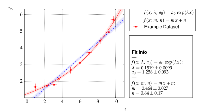
Output of example 1 - compare two models

The contour curves of the two fits are shown below and reflect the large correlations between the fit parameters. The right plot of the profile χ² curve shows that there is a slight deviation from the parabolic curve in the fist fit of a non-linear (exponential) function. For more details on the profiled χ² curve see the discussion of example 3, where the difference is more prominent.

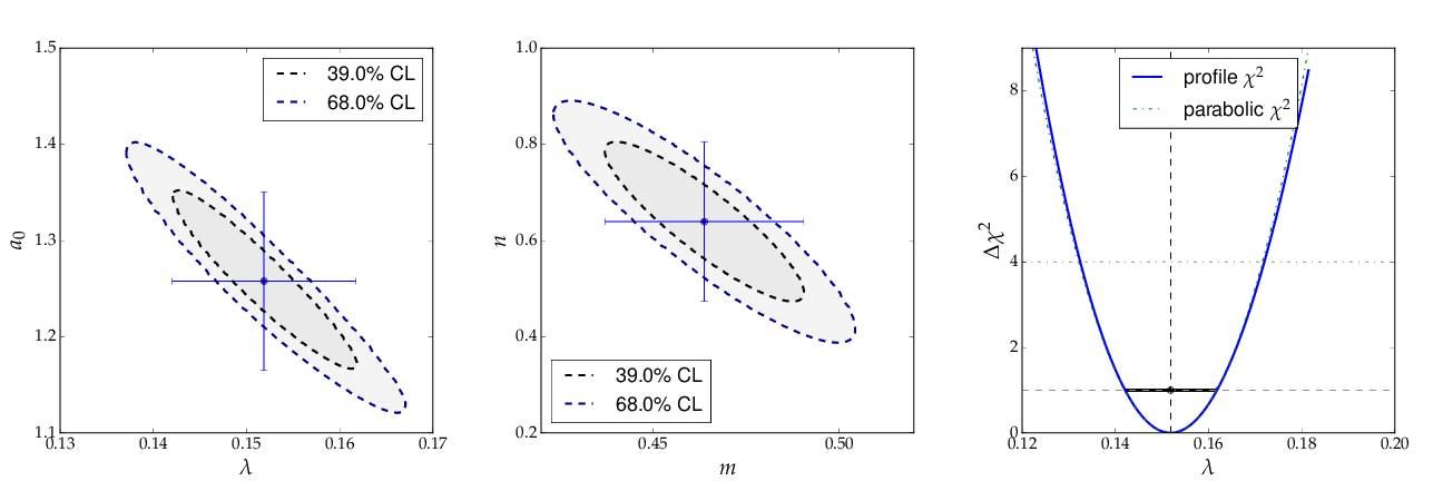
Contour curves and a profile χ² curve for the fits in example 1

Example 2 - two fits and models¶

Another typical use case consists of comparing two sets of measurements and the models derived from them. This is very similar to the previous example with minor modifications:

# import everything we need from kafe
import kafe

# additionally, import the model function we want to fit:
from kafe.function_library import linear_2par

# Initialize the Datasets
my_datasets = [kafe.Dataset(title="Example Dataset 1"),
               kafe.Dataset(title="Example Dataset 2")]

# Load the Datasets from files
my_datasets[0].read_from_file(input_file='dataset1.dat')
my_datasets[1].read_from_file(input_file='dataset2.dat')

# Create the Fits
my_fits = [kafe.Fit(dataset,
                    linear_2par,
                    fit_label="Linear regression " + dataset.data_label[-1])
           for dataset in my_datasets]

# Do the Fits
for fit in my_fits:
    fit.do_fit()

# Create the Plots
my_plot = kafe.Plot(my_fits[0], my_fits[1])
my_plot.plot_all()  # this time without any arguments, i.e. show everything

# Save the plots
my_plot.save('kafe_example2.pdf')

# Show the plots
my_plot.show()

This results in the following output:

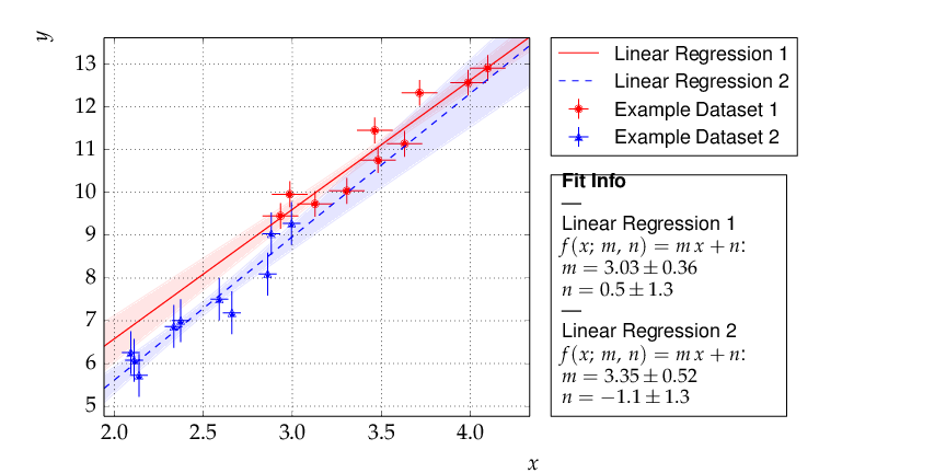
Output of example 2 - comparison of two linear fits.

Although the parameters extracted from the two data sets agree within errors, the uncertainty bands of the two functions do not overlap in the region where the data of Dataset 2 are located, so the data are most probably incompatible with the assumption of an underlying single linear model.

Example 3 - non-linear fit with non-parabolic errors¶

Very often, when the fit model is a non-linear function of the parameters, the χ² function is not parabolic around the minimum. A very common example of such a case is an exponential function parametrized as shown in the code fragment below. Minuit contains a special algorithm called MINOS, which returns the correct errors in this case as well. Instead of using the curvature at the minimum, MINOS follows the χ² function from the minimum to the point where it crosses the the value minimum+up, where up=1 corresponds to one standard deviation in χ² fits. During the scan of the χ² function at different values of each parameter, the minimum with respect to all other parameters in the fit is determined, thus making sure that all correlations among the parameters are taken into account. In case of a parabolic χ² function, the MINOS errors are identical to those obtained by the HESSE algorithm, but are typically larger or asymmetric in other cases.

The method do_fit() executes the MINOS algorithm after completion of a fit and prints the MINOS errors if the deviation from the parabolic result is larger than 5% .

A graphical visualization is provided by the method plot_profile() , which displays the profile χ² curve for the parameter with name or index passed as an argument to the method.

The relevant code fragments and the usage of the method plot_profile() are illustrated here:

import kafe

##################################
# Definition of the fit function #
##################################
# Set an ASCII expression for this function
@ASCII(x_name="t", expression="A0*exp(-t/tau)")
# Set some LaTeX-related parameters for this function
@LaTeX(name='A', x_name="t",
   parameter_names=('A_0', '\\tau{}'),
   expression="A_0\\,\\exp(\\frac{-t}{\\tau})")
@FitFunction
def exponential(t, A0=1, tau=1):
   return A0 * exp(-t/tau)


# Initialize the Dataset and load data from a file
my_dataset = kafe.Dataset(title="Example dataset",
                          axis_labels=['t', 'A'])
my_dataset.read_from_file(input_file='dataset.dat')

# Perform a Fit
my_fit = Fit(my_dataset, exponential)
my_fit.do_fit()

# Plot the results
my_plot = Plot(my_fit)
my_plot.plot_all()


# Create plots of the contours and profile chi-squared
contour = my_fit.plot_contour(0, 1, dchi2=[1.0, 2.3])
profile1 = my_fit.plot_profile(0)
profile2 = my_fit.plot_profile(1)

# Show the plots
my_plot.show()

The data points were generated using a normalization factor of A₀ = 1 and a lifetime τ = 1. The resulting fit output below demonstrates that this is well reproduced within uncertainties:

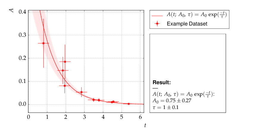
Output of example 3 - Fit of an exponential

The contour A₀ vs τ is, however, not an ellipse, as shown in the figure below. The profiled χ² curves are also shown; they deviate significantly from parabolas. The proper one-sigma uncertainty in the sense of a 68% confidence interval is read from these curves by determining the parameter values where the χ² curves cross the horizontal lines at a value of Δχ²=1 above the minimum. The two-sigma uncertainties correspond to the intersections with the horizontal line at Δχ²=4.

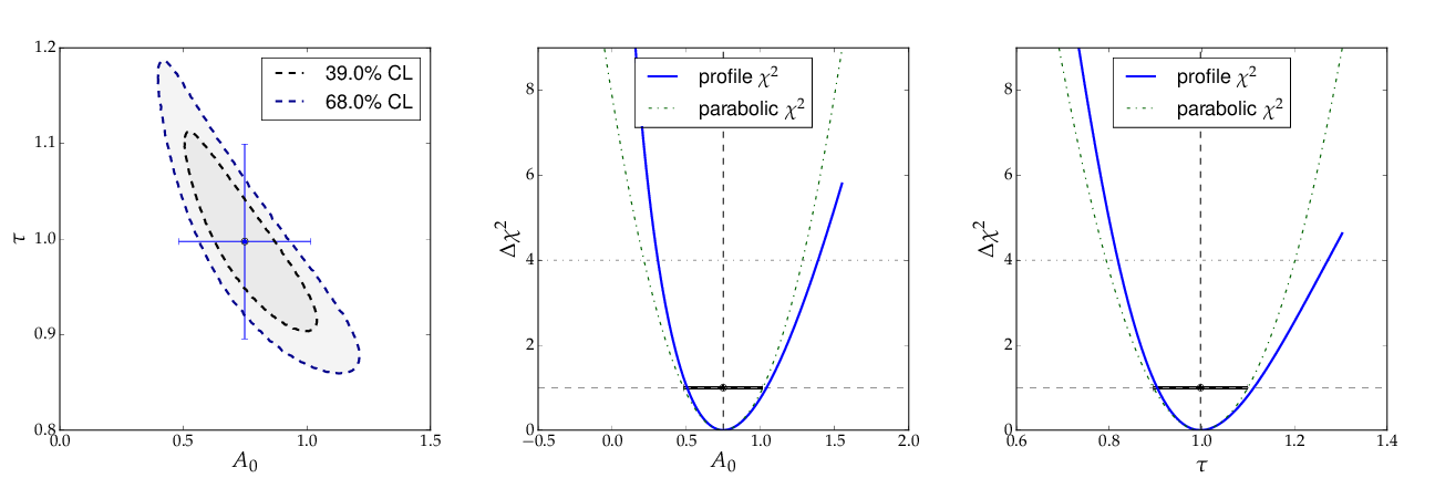
Contour and profile χ² curves of example 3

Note

A more parabolic behavior can be achieved by using the width parameter λ=1/τ in the parametrization of the exponential function.

Example 4 - average of correlated measurements¶

The average of a set of measurements can be considered as a fit of a constant to a set of input data. This example illustrates how correlated errors are handled in kafe. Measurements can have a common error, which may be absolute or relative, i. e. depend on the input value. In more complicated cases the full covariance matrix must be constructed.

kafe has a helper function, build_dataset() (in module dataset_tools), which aids in setting up the covariance matrix and transforming the input to the default format used by the Dataset and Fit classes. Two further helper functions in module file_tools aid in reading the appropriate information from data files.

The function parse_column_data() reads the input values and their

independent errors from one file, and optionally covariance matrices for the x and y axes from additional files. The field ordering is defined by a control string.
Another helper function, buildDataset_fromFile(), specifies

input values or blocks of input data from a single file with keywords.

The second version needs only very minimal additional user code, as illustrated here:

import kafe
from kafe.function_library import constant_1par
from kafe.file_tools import buildDataset_fromFile

# build Dataset from input file
fname = 'WData.dat'
curDataset = buildDataset_fromFile(fname)

# perform the Fit
curFit = kafe.Fit(curDataset, constant_1par)
curFit.do_fit()

# Plot the results
myPlot = kafe.Plot(curFit)
myPlot.plot_all()
myPlot.save("plot.pdf")
myPlot.show()

The input file is necessarily more complicated, but holds the full information on the data set in one place. Refer to the documentation of the function parse_general_inputfile() in module file_tools for a full description of the currently implemented keywords. The input file for the averaging example is here:

# Measurements of W boson mass (combined LEP2, 2013)
# ==================================================
# example to use parse_general_inputfile from kafe;
#  covariance matrix build from common errors
# ==

#  Metadata for plotting
*BASENAME WData
*TITLE measurements of the W boson mass
*xLabel number of measurement
*yLabel $m_\matrhm{W}$
*yUnit GeV/$c^2$

# x data need not be given for averaging

# ============================================================
#  Measurements of W mass by ALEPH, DELPHI, L3 and OPAL
#                              from from LEP2 Report Feb. 2013
#  common errors within channels
#                     2q2l: 0.021 GeV,
#                       4q: 0.044 GeV,
#     and between channels: 0.025 GeV
# ============================================================

*yData_SCOV

# W_mass   err      syst    sqrt of covariance matrix elements
#                              (as lower triangular matrix)
# 2q2l channel
  80.429   0.055    0.021
  80.339   0.073    0.021   0.021
  80.217   0.068    0.021   0.021 0.021
  80.449   0.058    0.021   0.021 0.021 0.021
# 4q  channel
  80.477   0.069    0.044   0.025 0.025 0.025 0.025 0.044
  80.310   0.091    0.044   0.025 0.025 0.025 0.025 0.044 0.044
  80.324   0.078    0.044   0.025 0.025 0.025 0.025 0.044 0.044 0.044
  80.353   0.068    0.044   0.025 0.025 0.025 0.025 0.044 0.044 0.044 0.044

Example 5 - non-linear multi-parameter fit (damped oscillation)¶

This example shows the fitting of a more complicated model function to data collected from a damped harmonic oscillator. In such non-linear fits, stetting the initial values is sometimes crucial to let the fit converge at the global minimum. The Fit object provides the method set_parameters() for this purpose. As the fit function for this problem is not a standard one, it is defined explicitly making use of the decorator functions available in kafe to provide nice type setting of the parameters. This time, the function parse_column_data() is used to read the input, which is given as separate columns with the fields

<time> <Amplitude> <error on time> <error on Amplitude>

Here is the example code:

import kafe
from numpy import exp, cos

#############################
# Model function definition #
#############################

# Set an ASCII expression for this function
@ASCII(x_name="t", expression="A0*exp(-t/tau)*cos(omega*t+phi)")
# Set some LaTeX-related parameters for this function
@LaTeX(name='A', x_name="t",
       parameter_names=('a_0', '\\tau{}', '\\omega{}', '\\varphi{}'),
       expression="a_0\\,\\exp(-\\frac{t}{\\tau})\,"
                  "\cos(\\omega{}\\,t+\\varphi{})")
@FitFunction
def damped_oscillator(t, a0=1, tau=1, omega=1, phi=0):
    return a0 * exp(-t/tau) * cos(omega*t + phi)

############
# Workflow #
############

# --- Load the experimental data from a file
my_dataset = parse_column_data(
    'oscillation.dat',
    field_order="x,y,xabserr,yabserr",
    title="Damped Oscillator",
    axis_labels=['Time $t$','Amplitude'])

# --- Create the Fit
my_fit = kafe.Fit(my_dataset, damped_oscillator)
# Set the initial values for the fit:
#                      a_0 tau omega phi
my_fit.set_parameters((1., 2., 6.28, 0.8))
my_fit.do_fit()

# --- Create and output the plots
my_plot = kafe.Plot(my_fit)
my_plot.plot_all()
my_fit.plot_correlations()  # plot all contours and profiles
my_plot.show()

This is the resulting output:

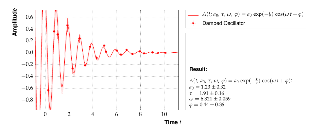
Example 5 - fit of the time dependence of the amplitude of a damped harmonic oscillator.

The fit function is non-linear, and, furthermore, there is not a single local minimum - e.g. a shift in phase of 180° corresponds to a change in sign of the amplitude, and valid solutions are also obtained for multiples of the base frequency. Checking of the validity of the fit result is therefore important. The method plot_correlations() provides the contours of all pairs of parameters and the profiles for each of the parameters and displays them in a matrix-like arrangement. Distorted contour-ellipses show whether the result is affected by near-by minima, and the profiles allow to correctly assign the parameter uncertainties in cases where the parabolic approximation is not precise enough.

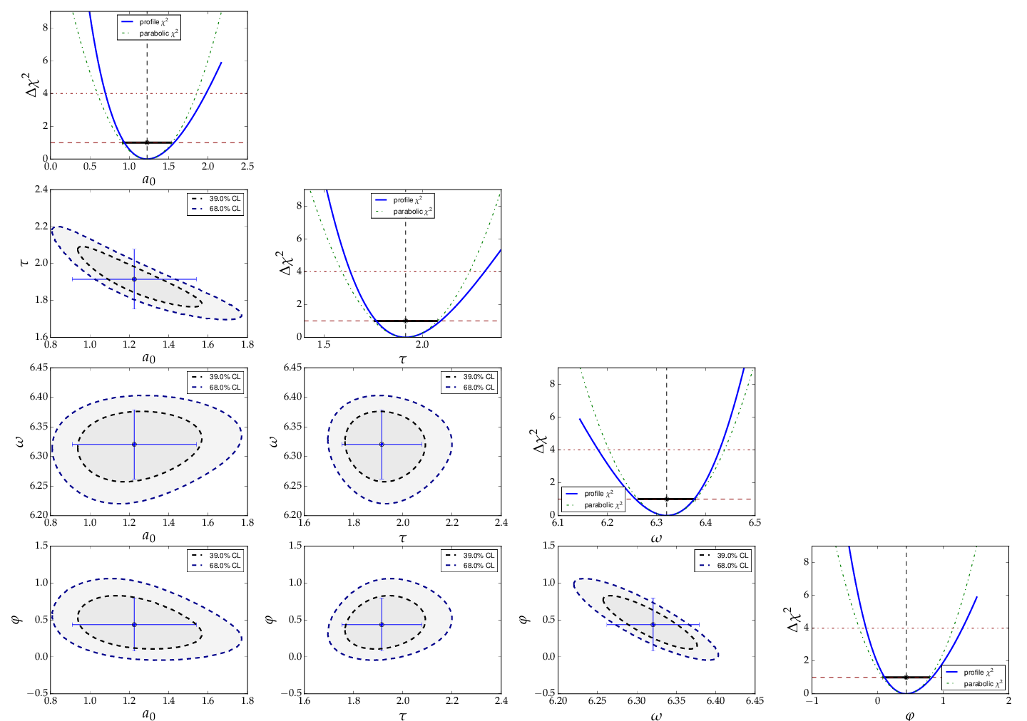
Confidence contours and profiles for example 5.

Example 6 - linear multi-parameter fit¶

This example is not much different from the previous one, except that the fit function, a standard fourth-degree polynomial from the module function_library, is modified to reflect the names of the problem given, and matplotlib functionality is used to influence the output of the plot, e.g. axis names and linear or logarithmic scale.

It is also shown how to circumvent a problem that often arises when errors depend on the measured values. For a counting rate, the (statistical) error is typically estimated as the square root of the (observed) number of entries in each bin. For large numbers of entries, this is not a problem, but for small numbers, the correlation between the observed number of entries and the error derived from it leads to a bias when fitting functions to the data. This problem can be avoided by iterating the fit procedure:

In a pre-fit, a first approximation of the model function is determined, which is then used to calculate the expected errors, and the original errors are replaced before performing the final fit.

Note

The numbers of entries in the bins must be sufficiently large to justify a replacement of the (asymmetric) Poisson uncertainties by the symmetric uncertainties implied by the χ²-method.

The implementation of this procedure needs accesses some more fundamental methods of the Dataset, Fit and FitFunction classes. The code shown below demonstrates how this can be done with kafe, using some of its lower-level, internal interfaces:

import kafe
import numpy as np

from kafe.function_library import poly4

# modify function's independent variable name to reflect its nature:
poly4.x_name = 'x=cos(t)'
poly4.latex_x_name = 'x=\\cos(\\theta)'

# Set the axis labels appropriately
my_plot.axis_labels = ['$\\cos(\\theta)$', 'counting rate']

# load the experimental data from a file
my_dataset = parse_column_data(
  'counting_rate.dat',
  field_order="x,y,yabserr",
  title="Counting Rate per Angle")

# -- begin pre-fit
# error for bins with zero contents is set to 1.
covmat = my_dataset.get_cov_mat('y')
for i in range(0, len(covmat)):
    if covmat[i, i] == 0.:
        covmat[i, i] = 1.
my_dataset.set_cov_mat('y', covmat)  # write it back

# Create the Fit
my_fit = kafe.Fit(my_dataset, poly4)

# perform an initial fit with temporary errors (minimal output)
my_fit.call_minimizer(final_fit=False, verbose=False)

# set errors using model at pre-fit parameter values:
#       sigma_i^2=cov[i, i]=n(x_i)
fdata = my_fit.fit_function.evaluate(my_fit.xdata,
                                     my_fit.current_parameter_values)
np.fill_diagonal(covmat, fdata)
my_fit.current_cov_mat = covmat  # write new covariance matrix
# -- end pre-fit - rest is as usual

my_fit.do_fit()
my_plot = kafe.Plot(my_fit)

# set the axis labels
my_plot.axis_labels = ['$\\cos(\\theta)$', 'counting rate']

# set scale ('linear'/'log')
my_plot.axes.set_yscale('linear')

my_plot.plot_all()
my_plot.show()

This is the resulting output:

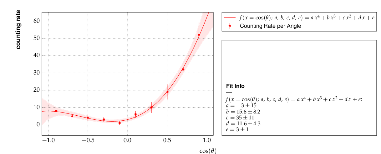
Output of example 6 - counting rate.

Example 7 - another non-linear multi-parameter fit (double-slit spectrum)¶

Again, not much new in this example, except that the model is now very non-linear, the intensity distribution of light after passing through a double-slit. The non-standard model definition again makes use of the decorator mechanism to provide nice output - the decorators (expressions beginning with @) can safely be omitted if LaTeX output is not needed. Setting of appropriate initial conditions is absolutely mandatory for this example, because there exist many local minima of the χ² function.

Another problem becomes obvious when carefully inspecting the fit function definition: only two of the three parameters g, b or k can be determined, and therefore one must be kept fixed, or an external constraint must be applied. Failing to do so will result in large, correlated errors on the parameters g, b and k as an indication of the problem.

Fixing parameters of a model function is achieved by the method fix_parameters(), and a constraint within a given uncertainty is achieved by the method constrain_parameters() of the Fit class.

Here are the interesting pieces of code:

import kafe
import numpy as np

from kafe import ASCII, LaTeX, FitFunction
from kafe.file_tools import parse_column_data

#############################
# Model function definition #
#############################

# Set an ASCII expression for this function
@ASCII(x_name="x", expression="I0*(sin(k/2*b*sin(x))/(k/2*b*sin(x))"
                              "*cos(k/2*g*sin(x)))^2")
# Set some LaTeX-related parameters for this function
@LaTeX(name='I', x_name="\\alpha{}",
       parameter_names=('I_0', 'b', 'g', 'k'),
       expression="I_0\\,\\left(\\frac{\\sin(\\frac{k}{2}\\,b\\,\\sin{\\alpha})}"
                  "{\\frac{k}{2}\\,b\\,\\sin{\\alpha}}"
                  "\\cos(\\frac{k}{2}\\,g\\,\\sin{\\alpha})\\right)^2")
@FitFunction
def double_slit(alpha, I0=1, b=10e-6, g=20e-6, k=1.e7):
    k_half_sine_alpha = k/2*np.sin(alpha)  # helper variable
    k_b = k_half_sine_alpha * b
    k_g = k_half_sine_alpha * g
    return I0 * (np.sin(k_b)/(k_b) * np.cos(k_g))**2

############
# Workflow #
############

# load the experimental data from a file
my_dataset = parse_column_data('double_slit.dat',
                field_order="x,y,xabserr,yabserr",
                title="Double Slit Data",
                axis_labels=['$\\alpha$', 'Intensity'] )

# Create the Fit
my_fit = kafe.Fit(my_dataset,
                  double_slit)

# Set the initial values for the fit
#                      I   b      g        k
my_fit.set_parameters((1., 20e-6, 50e-6, 9.67e6))
# fix one of the (redundant) parameters, here 'k'
my_fit.fix_parameters('k')

my_fit.do_fit()
my_plot = kafe.Plot(my_fit)
my_plot.plot_all()
my_plot.show()

If the parameter k in the example above has a (known) uncertainty, is is more appropriate to constrain it within its uncertainty (which may be known from an independent measurement or from the specifications of the laser used in the experiment). To take into account a wave number k known with a precision of 10000 the last line in the example above should be replaced by:

my_fit.constrain_parameters(['k'], [9.67e6], [1.e4])

This is the resulting output:

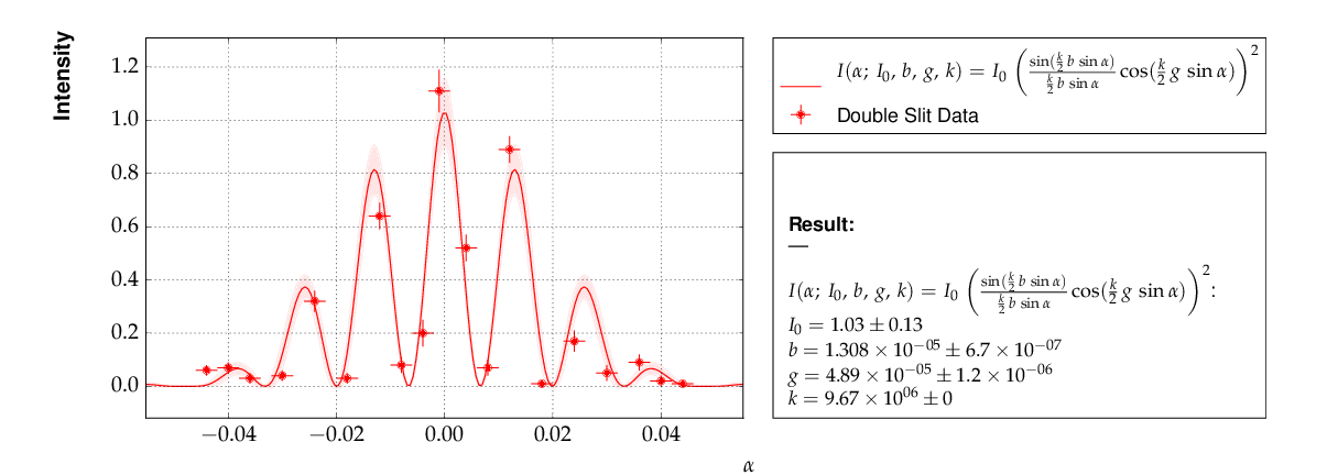
Example 7 - fit of the intensity distribution of light behind a double slit with fixed or constrained wave length.

Example 8 - fit of a Breit-Wigner resonance to data with correlated errors¶

This example illustrates how to define the data and the fit function in a single file - provided by the helper function buildFit_fromFile() in module file_tools. Parsing of the input file is done by the function parse_general_inputfile(), which had already been introduced in Example 4. The definition of the fit function as Python code including the kafe decorators in the input file, however, is new. The last key in the file defines the start values of the parameters and their initial ranges.

The advantage of this approach is the location of all data and the fit model in one place, which is strictly separated from the Python code. The Python code below is thus very general and can handle a large large variety of problems without modification (except for the file name, which could easily be passed on the command line):

import kafe
from kafe.file_tools import buildFit_fromFile

# initialize fit object from file
fname = 'LEP-Data.dat'
BWfit = buildFit_fromFile(fname)
BWfit.do_fit()

BWplot = kafe.Plot(BWfit)
BWplot.plot_all()
BWplot.save("plot.pdf")
BWplot.show()

The magic happens in the input file, which now has to provide all the information needed to perform the fit:

# Measurements of hadronic Z cross sections at LEP
# ------------------------------------------------
# this file is to be parsed with
#          kafe.file_tools.buildFit_fromFile()

#  Metadata for plotting
*TITLE  LEP Hadronic Cross Section ($\sigma^0_\mathrm{had}$)
*BASENAME example8_BreitWigner
*xLabel $E_{CM}$
*xUnit  $\mathrm{GeV}$
*yLabel $\sigma^0_{\mathrm{had}}$
*yUnit  $\mathrm{nb}$

#----------------------------------------------------------------------
# DATA: average of hadronic cross sections measured by
#  ALEPH, DELPHI, L3 and OPAL around 7 energy points at the Z resonance
#----------------------------------------------------------------------

# CMenergy E err
*xData
   88.387  0.005
   89.437  0.0015
   90.223  0.005
   91.238  0.003
   92.059  0.005
   93.004  0.0015
   93.916  0.005

# Center-of-mass energy has a common uncertainty
*xAbsCor 0.0017

# sig^0_h  sig err     #  rad.cor  sig_h measured
*yData
   6.803   0.036      #  1.7915    5.0114
   13.965  0.013      #  4.0213    9.9442
   26.113  0.075      #  7.867    18.2460
   41.364  0.010      #  10.8617  30.5022
   27.535  0.088      #  3.9164   23.6187
   13.362  0.015      # -0.6933   14.0552
    7.302  0.045      # -1.8181    9.1196

# cross-sections have a common relative error
*yRelCor 0.0007

*FITLABEL Breit-Wigner-Fit \, {\large{(with~s-dependent~width)}}

*FitFunction
# Breit-Wigner with s-dependent width
@ASCII(name='sigma', expression='s0*x^2*G^2/[(E^2-M^2)^2+(E^4*G^2/M^2)]')
@LaTeX(name='\sigma', parameter_names=('\\sigma^0', 'M_Z','\\Gamma_Z'),
expression='\\frac{\\sigma^0\\, M_Z^2\\Gamma^2}'
                 '{((E^2-M_Z^2)^2+(E^4\\Gamma^2 / M_Z^2))}')
@FitFunction
def BreitWigner(E, s0=41.0, M=91.2, G=2.5):
    return s0*E*E*G*G/((E*E-M*M)**2+(E**4*G*G/(M*M)))


*InitialParameters  # initial values and range
41.  0.5
91.2 0.1
2.5  0.1

#---------------------------------------------------------------------------
#### official results (LEP Electroweak Working Group):
#### s0=41.540+/-0.037nb  M=91.1875+/-0.0021GeV/c^2  G=2.4952+/-0.0023 GeV
####  uses all decay modes of the Z and full cross-section list
#---------------------------------------------------------------------------

Here is the output:

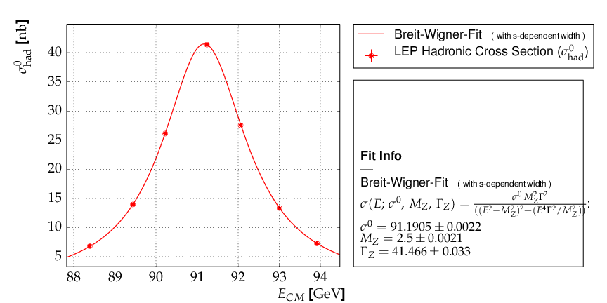
Output of example 8 - Fit of a Breit-Wigner function.

This example also contains a code snippet demonstrating how to plot contours by calling the Fit object’s plot_contour() method. This is the code:

# plot pairs of contours at 1 sigma, 68%, 2 sigma and 95%
cont_fig1 = BWfit.plot_contour(0, 1, dchi2=[1.0, 2.3, 4.0, 5.99])
cont_fig2 = BWfit.plot_contour(0, 2, dchi2=[1.0, 2.3, 4.0, 5.99])
cont_fig3 = BWfit.plot_contour(1, 2, dchi2=[1.0, 2.3, 4.0, 5.99])

# save to files
cont_fig1.savefig("kafe_BreitWignerFit_contour12.pdf")
cont_fig2.savefig("kafe_BreitWignerFit_contour13.pdf")
cont_fig3.savefig("kafe_BreitWignerFit_contour23.pdf")

The resulting pictures show that parameter correlations are relatively small:

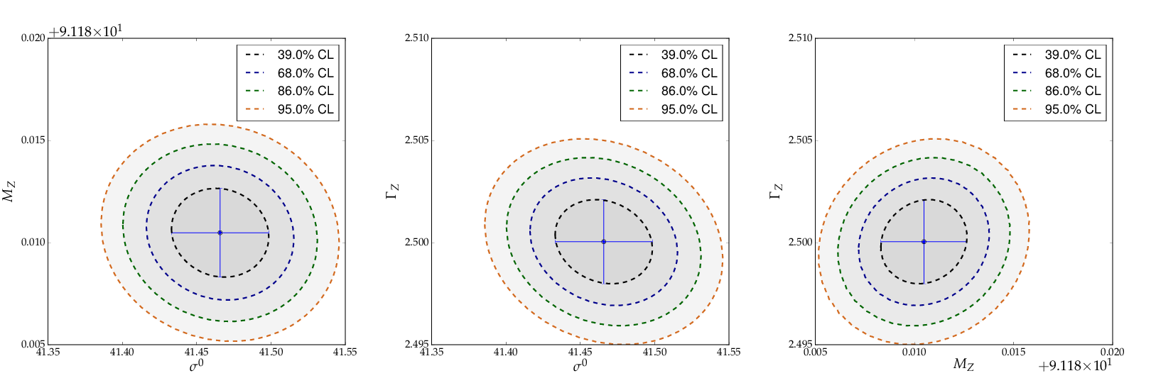
Contours generated in example 8 - Fit of a Breit-Wigner function.

Example 9 - fit of a function to histogram data¶

This example brings us to the limit of what is currently possible with kafe. Here, the data represent the center of a histogram bins ad the number of entries, $n_i$ , in each bin. The (statistical) error is typically estimated as the square root of the (observed) number of entries in each bin. For large numbers of entries, this is not a problem, but for small numbers, especially for bins with 0 entries, the correlation between the observed number of entries and the error derived from it leads to a bias when fitting functions to the histogram data. In particular, bins with zero entries cannot be handled in the χ²-function, and are typically omitted to cure the problem. However, a bias remains, as bins with downward fluctuations of the observed numbers of events get assigned smaller errors and hence larger weights in the fitting procedure - leading to the aforementioned bias.

These problems are avoided by using a likelihood method for such use cases, where the Poisson distribution of the uncertainties and their dependence on the values of the fit model is properly taken into account. However, the χ²-method can be saved to some extend if the fitting procedure is iterated. In a pre-fit, a first approximation of the model function is determined, where the error in bins with zero entries is set to one. The model function determined from the pre-fit is then used to calculate the expected errors for each bin, and the original errors are replaced before performing the final fit.

Note

The numbers of entries in the bins must be sufficiently large to justify a replacement of the (asymmetric) Poisson uncertainties by the symmetric uncertainties implied by the χ²-method.

The code shown below demonstrates how to get a grip on such more complex procedures with more fundamental methods of the Dataset, Fit and FitFunction classes:

import kafe
import numpy as np

from kafe.function_library import gauss


# Load Dataset from file
hdataset = kafe.Dataset(title="Data for example 9",
                        axis_labels=['x', 'entries'])
hdataset.read_from_file('hdataset.dat')

# error for bins with zero contents is set to 1.
covmat = hdataset.get_cov_mat('y')
for i in range(0, len(covmat)):
    if covmat[i, i] == 0.:
        covmat[i, i] = 1.
hdataset.set_cov_mat('y', covmat) # write it back

# Create the Fit instance
hfit = kafe.Fit(hdataset, gauss, fit_label="Fit of a Gaussian to histogram data")

# perform an initial fit with temporary errors (minimal output)
hfit.call_minimizer(final_fit=False, verbose=False)

#re-set errors using model at pre-fit parameter values:
#        sigma_i^2=cov[i, i]=n(x_i)
fdata=hfit.fit_function.evaluate(hfit.xdata, hfit.current_parameter_values)
np.fill_diagonal(covmat, fdata)
hfit.current_cov_mat = covmat  # write back new covariance matrix

# now do final fit with full output
hfit.do_fit()

hplot = kafe.Plot(hfit)
hplot.plot_all()
hplot.show()

Here is the output, which shows that the parameters of the standard normal distribution, from which the data were generated, are reproduced well by the fit result:

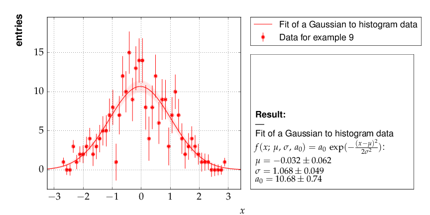
Output of example 9 - Fit of a Gaussian distribution to histogram data

Example 10 - plotting with kafe: properties of a Gauss curve¶

This example shows how to access the kafe plot objects to annotate plots with matplotlib functionality.

A dummy object Dataset is created with points lying exactly on a Gaussian curve. The Fit will then converge toward that very same Gaussian. When plotting, the data points used to “support” the curve can be omitted.

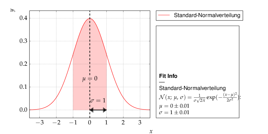
Output of example 10 - properties of a Gauss curve.

Examples 11 and 12 - approaches to fitting several models to multivariate data¶

The premise of this example is deceptively simple: a series of voltages is applied to a resistor and the resulting current is measured. The aim is to fit a model to the collected data consisting of voltage-current pairs and determine the resistance $R$ .

According to Ohm’s Law, the relation between current and voltage is linear, so a linear model can be fitted. However, Ohm’s Law only applies to an ideal resistor whose resistance does not change, and the resistance of a real resistor tends to increase as the resistor heats up. This means that, as the applied voltage gets higher, the resistance changes, giving rise to nonlinearities which are ignored by a linear model.

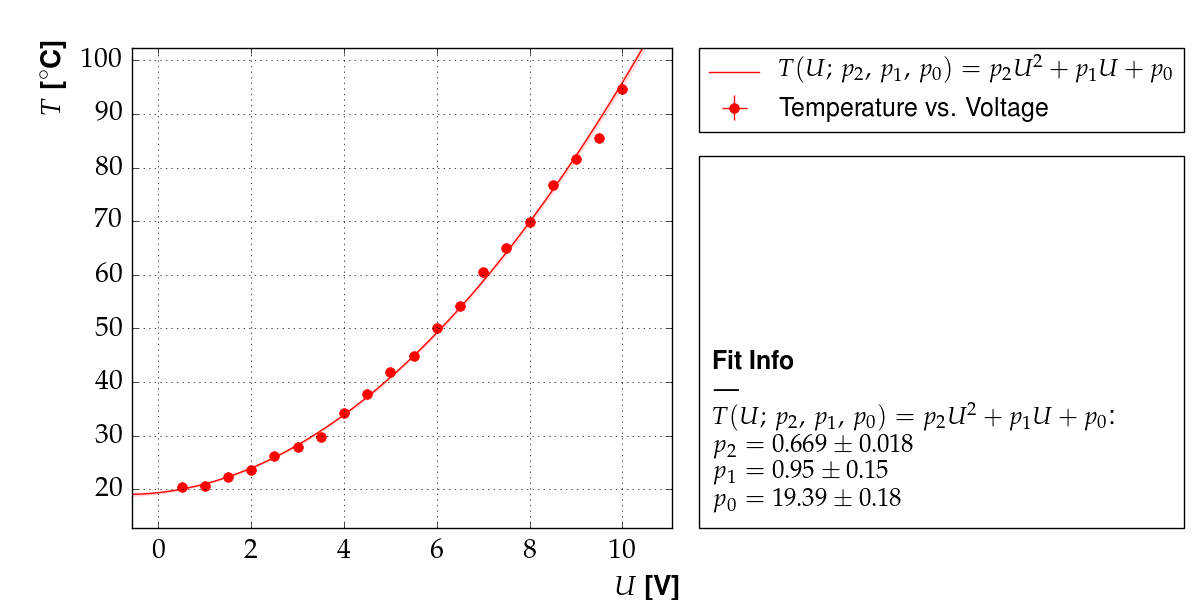
To get a hold on this nonlinear behavior, the model must take the temperature of the resistor into account. Thus, the temperature is also recorded for every data point. The data thus consists of triples, instead of the usual “xy” pairs, and the relationship between temperature and voltage must be modeled in addition to the one between current and voltage.

Here, the dependence $T(U)$ is taken to be quadratic, with some coefficients $p_0$ , $p_1$ , and $p_2$ :

$T(U) = p_2 U^2 + p_1 U + p_0$

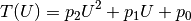
This model is based purely on empirical observations. The $I(U)$ dependence is more complicated, but takes the “running” of the resistance with the temperature into account:

$I(U) = \frac{U}{R_0 (1 + t \cdot \alpha_T)}$

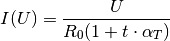
In the above, $t$ is the temperature in degrees Celsius, $\alpha_T$ is an empirical “heat coefficient”, and $R_0$ is the resistance at 0 degrees Celsius, which we want to determine.

In essence, there are two models here which must be fitted to the $I(U)$ and $T(U)$ data sets, and one model “incorporates” the other in some way.

Example 11: constraining parameters¶

There are several ways to achieve this with kafe. The method chosen here is to fit the empirical $T(U)$ model to the $T(U)$ data and extract the parameter estimated $p_i$ , along with their uncertainties and correlations.

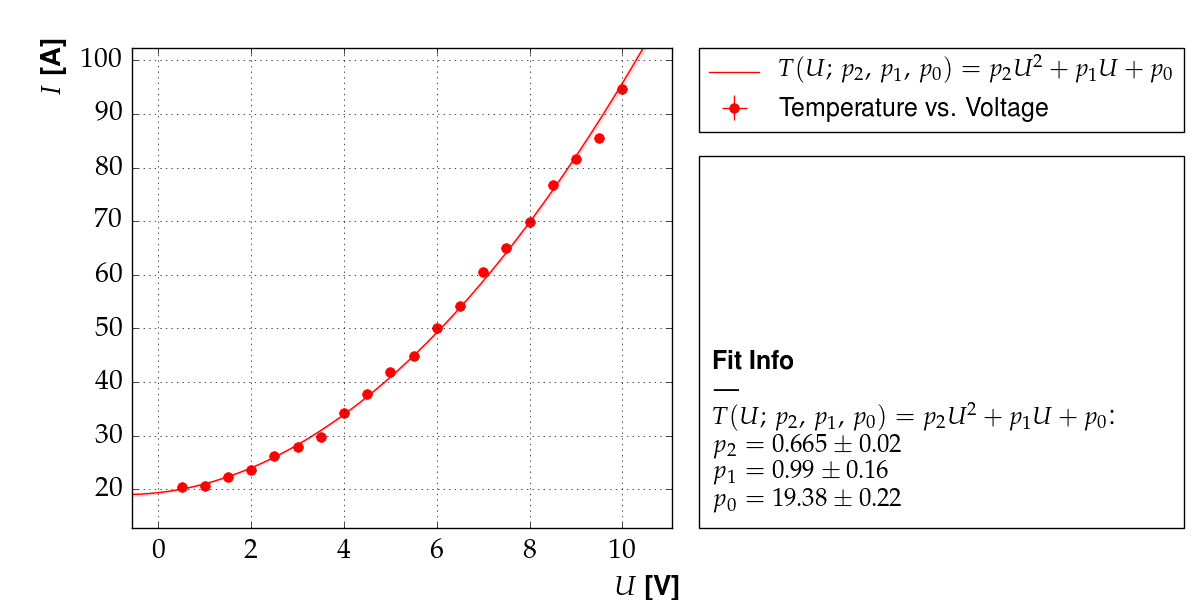
Output of example 11: Temperature as a function of voltage

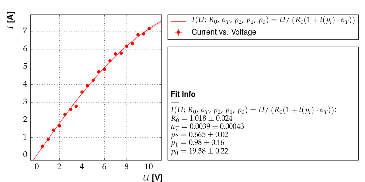
Output of example 11: Current as a function of voltage

Then, a fit of the $I(U)$ model is performed to the $I(U)$ data, while keeping the parameters constrained around the previously obtained values.

This approach is very straightforward, but it has the disadvantage that not all data is used in a optimal way. Here, for example, the $I(U)$ data is not taken into account at all when fitting $T(U)$ .

A more flexible approach, the “multi-model” fit, is demonstrated in example 12.

Example 12: multi-model fit¶

There are several ways to achieve this with kafe. The method chosen here is to use the Multifit functionality to fit both models simultaneously to the $T(U)$ and $I(U)$ datasets.

Output of example 12: Temperature as a function of voltage

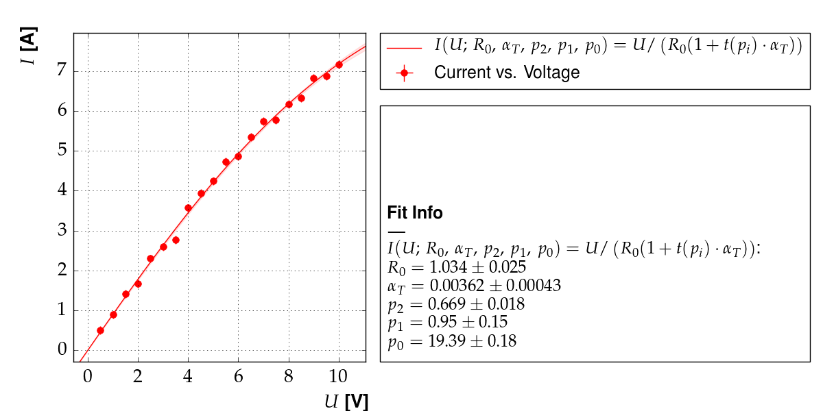
Output of example 12: Current as a function of voltage

In general, this approach yields different results than the one using parameter constraints, which is demonstrated in example 11.